Proposing a Successful Film

Data

This project uses data made available by Internet Movie Database (IMDb). While I did intially use the full data set in my analysis, I switched over to using a sub-sampled pre-processed data because my computer was struggling to handle the full data.

library(tidyverse)
library(dplyr)
library(tidyr)
library(ggplot2)
library(gt)

get_imdb_file <- function(fname){
  fname_ext <- paste0(fname, ".csv.zip")
  as.data.frame(readr::read_csv(fname_ext, lazy=FALSE))
}

NAME_BASICS <- get_imdb_file("name_basics_small")
TITLE_BASICS     <- get_imdb_file("title_basics_small")
TITLE_EPISODES <- get_imdb_file("title_episodes_small")
TITLE_RATINGS <- get_imdb_file("title_ratings_small")
TITLE_CREW <- get_imdb_file("title_crew_small")
TITLE_PRINCIPALS <- get_imdb_file("title_principals_small")

Below, I am converting the birth year and death year to numeric data types.

NAME_BASICS <- NAME_BASICS |>
  mutate(birthYear = as.numeric(birthYear), # numeric birth years
         deathYear = as.numeric(deathYear))

With that, the data I am using has been narrowed down significantly to a smaller and manageable sub sample.

Name Basics

Display Code

library(DT)
library(dplyr)

sample_n(NAME_BASICS, 1000) |>
  DT::datatable()

Title Basics

Display Code

sample_n(TITLE_BASICS, 1000) |>
  DT::datatable()

Title Crew

Display Code

sample_n(TITLE_CREW, 1000) |>
  DT::datatable()

Title Episodes

Display Code

sample_n(TITLE_EPISODES, 1000) |>
  DT::datatable()

Title Ratings

Display Code

sample_n(TITLE_RATINGS, 1000) |>
  DT::datatable()

Title Principals

Display Code

sample_n(TITLE_PRINCIPALS, 1000) |>
  DT::datatable()

Preliminary Exploration

1. How many movies are in our data set? How many TV series? How many TV episodes?

Display Code

library(gt)
TITLE_BASICS |>
  group_by(titleType) |>
  filter(titleType %in% c("movie", "tvSeries", "tvEpisode" )) |>
  summarise(count = n()) |>
  gt() |> # create a display table
  tab_header(
    title = "Number of Title Types"
  ) |>
  cols_label( # display column names
    titleType = "Type",
    count = "Count"
  )

Number of Title Types
Type	Count
movie	131662
tvEpisode	155722
tvSeries	29789

2. Who is the oldest living person in our data set?

Display Code

NAME_BASICS |> 
  filter(is.na(deathYear)) |> # filter for those without a deathYear
  arrange(birthYear) |> 
  slice(1) |>
  gt() |> # create a display table
  cols_label( # display column names
    primaryName = "Name",
    birthYear = "Birth Year"
  )

nconst	Name	Birth Year	deathYear	primaryProfession	knownForTitles
nm5671597	Robert De Visée	1655	NA	composer,soundtrack	tt2219674,tt1743724,tt0441074,tt14426058

The results of this first query says Robert De Visee but Robert was born in 1655, which does not make sense at all. A quick Google search says that the oldest person alive in 2024 is 116. Given that, let us filter for people born after 1914.

Display Code

NAME_BASICS |> 
  filter(is.na(deathYear)) |> # filter for those without a deathYear
  filter(birthYear>=1914) |>
  arrange(birthYear) |> 
  slice(1)

     nconst    primaryName birthYear deathYear primaryProfession
1 nm0029349 Antonio Anelli      1914        NA             actor
                           knownForTitles
1 tt0072364,tt0068416,tt0065460,tt0068973

Let’s perform a sanity check by confirming online. The internet says Antonio Anelli died on 12 May 1977.

Display Code

NAME_BASICS |> 
  filter(is.na(deathYear)) |> # filter for those without a deathYear
  filter(birthYear>=1916) |>
  arrange(birthYear) |> 
  slice(1)

     nconst primaryName birthYear deathYear                   primaryProfession
1 nm0048527   Ivy Baker      1916        NA costume_department,costume_designer
                           knownForTitles
1 tt0041959,tt0054518,tt0066344,tt0042522

Ivy Baker born in 1916 and her bio on IMDb does not have a death year.

To be safe, let’s check for a year before 1916 and look at 1915.

Display Code

NAME_BASICS |> 
  filter(is.na(deathYear)) |> # filter for those without a deathYear
  filter(birthYear>=1915) |>
  arrange(birthYear) |> 
  slice(1)

     nconst    primaryName birthYear deathYear     primaryProfession
1 nm0015296 Akhtar-Ul-Iman      1915        NA writer,actor,director
                           knownForTitles
1 tt0059893,tt0175450,tt0060689,tt0158587

The result says Akhtar-Ul-Iman but according to Wikipedia, he died on March 9, 1996.

3. There is one TV Episode in this data set with a perfect 10/10 rating and 200,000 IMDb ratings.

Display Code

TITLE_RATINGS |> 
  left_join(TITLE_EPISODES, by = "tconst") |> # join using tconst
  filter(averageRating == 10.0 & numVotes >= 200000) |> # filter by averageRating and numVotes
  left_join(TITLE_BASICS, by = "tconst") |> # join using tconst
  left_join(TITLE_BASICS, join_by("parentTconst" == "tconst")) |>
  select(primaryTitle.y, primaryTitle.x, averageRating, numVotes) |> # select just the title, average rating, and number of votes
  gt() |> # create a display table
  tab_header(
    title = "Perfect TV Episode"
  ) |>
  cols_label( # display column names
    primaryTitle.y = "TV Show",
    primaryTitle.x = "Episode",
    averageRating = "Average Rating",
    numVotes = "Number of Votes"
  )

Perfect TV Episode
TV Show	Episode	Average Rating	Number of Votes
Breaking Bad	Ozymandias	10	227589

4. What four projects is the actor Mark Hammill most known for?

Display Code

library(tidyr)
NAME_BASICS |> 
  filter(primaryName == "Mark Hamill") |> 
  select(knownForTitles) |> 
  separate_rows(knownForTitles, sep = ",") |>  # Split by comma to make each knownForTitle a row
  left_join(TITLE_BASICS, by = c("knownForTitles" = "tconst")) |> # join to TITLE_BASICS on tconst
  select(primaryTitle) |> 
  head(4) |>
  gt() |> # create a display table
  tab_header(
    title = "Titles Mark Hammil is Known For"
  ) |>
  cols_label( # display column names
    primaryTitle = "Title"
  )

Titles Mark Hammil is Known For
Title
Star Wars: Episode IV - A New Hope
Star Wars: Episode VIII - The Last Jedi
Star Wars: Episode V - The Empire Strikes Back
Star Wars: Episode VI - Return of the Jedi

5. What TV series, with more than 12 episodes, has the highest average rating?

Display Code

# Find the highest-rated TV series with more than 12 episodes
# tt15613780        9.7           318 Craft Games

TITLE_BASICS |>
  filter(titleType == "tvSeries") |>
  right_join(TITLE_EPISODES, by = c("tconst" = "parentTconst")) |>
  group_by(tconst) |>
  mutate(episode_count = n()) |>
  ungroup() |>
  filter(episode_count > 12) |>
  left_join(TITLE_RATINGS, by = "tconst") |>
  arrange(desc(averageRating)) |>
  select(primaryTitle, averageRating, episode_count) |>
  head(1) |>
  gt() |> # create a display table
  tab_header(
    title = "Highest-Rated TV Series with More Than 12 Episodes"
  ) |>
  cols_label( # display column names
    primaryTitle = "TV Series",
    averageRating = "Average Rating",
    episode_count = "Number of Episodes"
  )

Highest-Rated TV Series with More Than 12 Episodes
TV Series	Average Rating	Number of Episodes
Craft Games	9.7	318

6. Is it true that episodes from later seasons of Happy Days have lower average ratings than the early seasons? The TV series Happy Days (1974-1984) gives us the common idiom “jump the shark”. The phrase comes from a controversial fifth season episode (aired in 1977) in which a lead character literally jumped over a shark on water skis. Idiomatically, it is used to refer to the moment when a once-great show becomes ridiculous and rapidly looses quality.

First, I’m finding the tconst for Happy Days.

Display Code

TITLE_BASICS |>
  filter(originalTitle == "Happy Days") |>
  filter(titleType == "tvSeries") |>
  filter(startYear == "1974") |>
  select(tconst) # find the tconst for Happy Days

     tconst
1 tt0070992

We can see below that seasons 1 through 4 do well in terms of average rating. Aside from season 11, the seasons after season 5 are all in the bottom half of ratings. Meanwhile, season 3 has the highest rating of 7.7.

Display Code

TITLE_EPISODES |> 
  filter(parentTconst == "tt0070992") |> 
  left_join(TITLE_RATINGS, join_by("tconst" )) |> 
  group_by(seasonNumber) |> 
  summarize(avg_rating = mean(averageRating, na.rm = TRUE)) |> 
  mutate(seasonNumber = as.numeric(seasonNumber)) |>
  select(seasonNumber, avg_rating) |>
  arrange(desc(avg_rating)) |> # arrange by average rating in descending order
  gt() |> # create a display table
  tab_header(
    title = "Ratings for Happy Days by Season"
  ) |>
  cols_label( # display column names
    seasonNumber = "Season",
    avg_rating = "Average Rating"
  )

Ratings for Happy Days by Season
Season	Average Rating
3	7.700000
2	7.691304
1	7.581250
4	7.428000
11	7.333333
6	7.018750
5	7.000000
10	6.700000
9	6.400000
7	6.333333
8	5.400000

In the plot below, we see that there is a indeed a dip in ratings in the later seasons of the show.

Display Code

season_ratings <- TITLE_EPISODES |> 
  filter(parentTconst == "tt0070992") |> 
  left_join(TITLE_RATINGS, join_by("tconst" )) |> 
  group_by(seasonNumber) |> 
  summarize(avg_rating = mean(averageRating, na.rm = TRUE)) |> 
  mutate(seasonNumber = as.numeric(seasonNumber)) |>
  select(seasonNumber, avg_rating) |>
  arrange(desc(seasonNumber)) # arrange by season in descending order

library(ggplot2)
# Bar chart of average ratings by season 
ggplot(season_ratings, aes(x = seasonNumber, y = avg_rating)) +
  geom_bar(stat = "identity", fill = "steelblue") +
  labs(title = "Average Ratings of Happy Days by Season",
       x = "Season Number",
       y = "Average Rating") +
  ylim(0,10) +
  scale_x_continuous(breaks = seq(1, 11, by = 1)) +
  geom_text(aes(label=round(avg_rating, digits = 1)), vjust=0)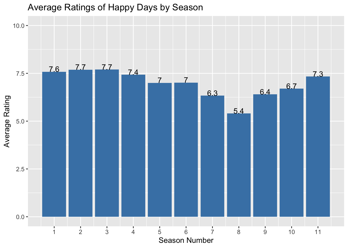

Quantifying Success

Next, I will be designing a ‘success’ measure for IMDb entries, reflecting both quality and broad popular awareness. I will be adding this measure to the TITLE_RATINGS table.

Initially, I did a composite score of averageRating and numVotes to consider both quality and popularity. I then divided this by the max possible score in the data population.
(averageRating x numVotes ) / (max(averageRating) x max(numVotes))

Display Code

TITLE_RATINGS$score <- (TITLE_RATINGS$averageRating * TITLE_RATINGS$numVotes) /
  (max(TITLE_RATINGS$averageRating) * max(TITLE_RATINGS$numVotes))
# plot to see spread/distribution
ggplot(TITLE_RATINGS, aes(x=score)) + geom_histogram()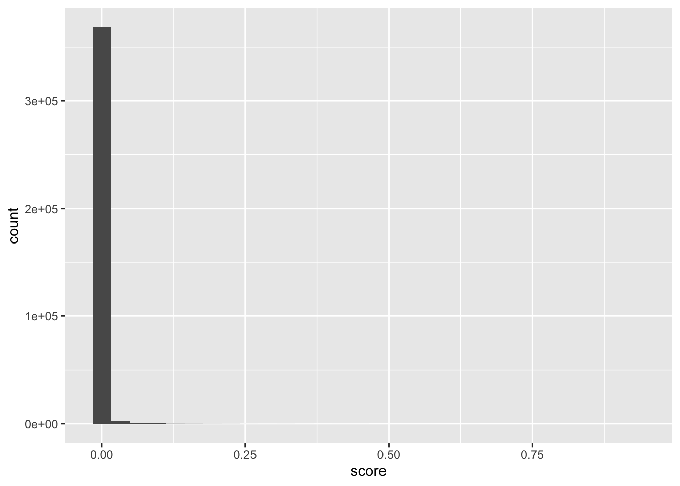

I don’t want the number of votes to throw off the score. Let’s use log on numVotes and maybe I want to give more weight to the rating than the number of votes. (0.6 x averageRating + 0.4 x log(numVotes)) / (0.6 x max(averageRating) + 0.4 x log(max(numVotes)))

Display Code

TITLE_RATINGS$success_score <- (.6*TITLE_RATINGS$averageRating + .4*log(TITLE_RATINGS$numVotes)) /
  (.6*max(TITLE_RATINGS$averageRating) + .4*log(max(TITLE_RATINGS$numVotes)))

ggplot(TITLE_RATINGS, aes(x=success_score)) + geom_histogram() +
  labs(title = "Success Score Distribution",
       x = "Success Score",
       y = "Frequency")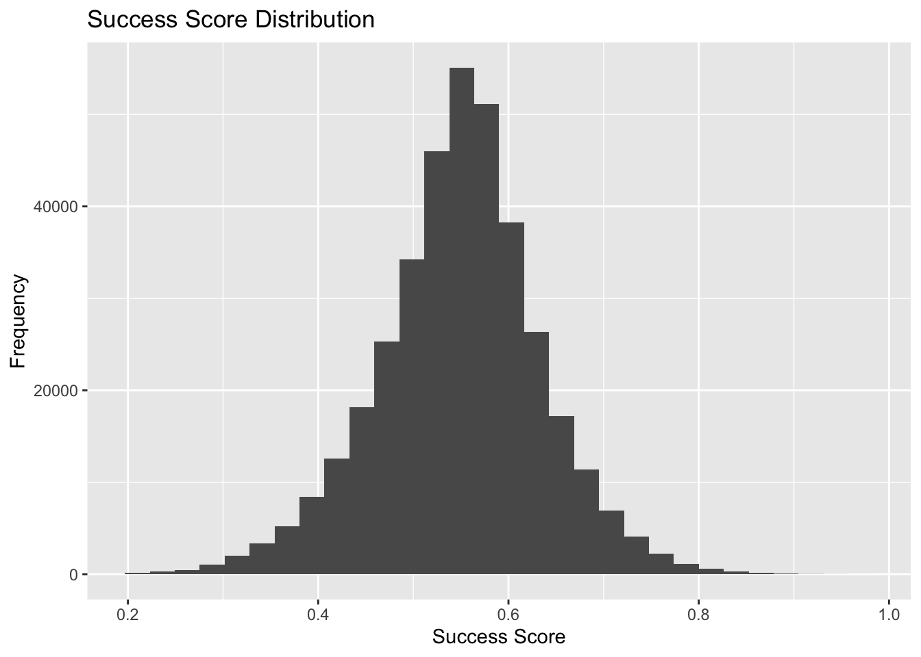

Now that there is a success score, let’s validate the metric with a number of tests and see how it holds up. First, I’m confirming that the the top 5-10 movies based on my metric were indeed box office successes.

Display Code

TITLE_RATINGS |> 
  arrange(desc(success_score)) |>  
  left_join(TITLE_BASICS, join_by("tconst" )) |> 
  filter(titleType == 'movie') |> 
  select(primaryTitle, success_score, averageRating, numVotes) |>
  head(10) |>
  gt() |> # create a display table
  tab_header(
    title = "Most Successful Movies"
  ) |>
  cols_label( # display column names
    primaryTitle = "Title",
    success_score = "Success Score",
    averageRating = "Average Rating",
    numVotes = "Number of Votes"
  )

Most Successful Movies
Title	Success Score	Average Rating	Number of Votes
The Shawshank Redemption	0.9648769	9.3	2942823
The Dark Knight	0.9495972	9.0	2922922
The Godfather	0.9477853	9.2	2051186
The Lord of the Rings: The Return of the King	0.9371353	9.0	2013824
Pulp Fiction	0.9359758	8.9	2260017
Inception	0.9355887	8.8	2595555
Fight Club	0.9326142	8.8	2374722
The Lord of the Rings: The Fellowship of the Ring	0.9326021	8.9	2043202
Forrest Gump	0.9315685	8.8	2301630
Schindler's List	0.9267397	9.0	1475891

Next, let’s use the success metric to find movies with large numbers of IMDb votes that score poorly and confirm that they are indeed of low quality.

Display Code

summary(TITLE_RATINGS$numVotes)

   Min. 1st Qu.  Median    Mean 3rd Qu.    Max. 
    100     165     332    4022     970 2942823

Display Code

TITLE_RATINGS |> 
  arrange(success_score) |> # arrage ascending
  left_join(TITLE_BASICS, join_by("tconst" )) |> 
  filter(titleType == 'movie') |>
  filter(numVotes >= 4022) |> # Mean numVotes is 4022
  select(primaryTitle, success_score, averageRating, numVotes) |>
  head(5) |> # select bottom 5
  gt() |> # create a display table
  tab_header(
    title = "Least Successful Movies"
  ) |>
  cols_label( # display column names
    primaryTitle = "Title",
    success_score = "Success Score",
    averageRating = "Average Rating",
    numVotes = "Number of Votes"
  )

Least Successful Movies
Title	Success Score	Average Rating	Number of Votes
Debt Fees	0.3537226	1.4	4791
Desh Drohi	0.3544280	1.2	6605
321 Action	0.3589619	1.0	10210
Jurassic Shark	0.3600881	1.5	4988
Birdemic 2: The Resurrection	0.3608768	1.5	5107

Now, to check in with the people, I will choose prestige actors or directors and confirm that they have many projects with high scores on my success metric.

Hayao Miyazaki

Display Code

NAME_BASICS |>
  filter(primaryName == 'Rob Reiner') |>
  separate_longer_delim(knownForTitles, ",") |> 
  left_join(TITLE_BASICS, by = c("knownForTitles" = "tconst")) |> 
  left_join(TITLE_RATINGS, by = c("knownForTitles" = "tconst")) |>
  select(primaryName, primaryTitle, success_score, averageRating, numVotes) |>
  arrange(desc(success_score)) |>
  gt() |> # create a display table
  tab_header(
    title = "Rob Reiner Project Scores"
  ) |>
  cols_label( # display column names
    primaryName = "Name",
    primaryTitle = "Title",
    success_score = "Success Score",
    averageRating = "Average Rating",
    numVotes = "Number of Votes"
  )

Rob Reiner Project Scores
Name	Title	Success Score	Average Rating	Number of Votes
Rob Reiner	The Wolf of Wall Street	0.8897217	8.2	1620302
Rob Reiner	This Is Spinal Tap	0.7948250	7.9	148925
Rob Reiner	All in the Family	0.7512242	8.4	19106
Rob Reiner	The Story of Us	0.6399937	6.0	25148

Christopher Nolan

Display Code

NAME_BASICS |>
  filter(primaryName == 'Christopher Nolan') |>
  separate_longer_delim(knownForTitles, ",") |> 
  left_join(TITLE_BASICS, by = c("knownForTitles" = "tconst")) |> 
  left_join(TITLE_RATINGS, by = c("knownForTitles" = "tconst")) |>
  filter(!is.na(primaryTitle)) |>
  select(primaryName, primaryTitle, success_score, averageRating, numVotes) |>
  arrange(desc(success_score)) |>
  gt() |> # create a display table
  tab_header(
    title = "Christopher Nolan Project Scores"
  ) |>
  cols_label( # display column names
    primaryName = "Name",
    primaryTitle = "Title",
    success_score = "Success Score",
    averageRating = "Average Rating",
    numVotes = "Number of Votes"
  )

Christopher Nolan Project Scores
Name	Title	Success Score	Average Rating	Number of Votes
Christopher Nolan	Inception	0.9355887	8.8	2595555
Christopher Nolan	Interstellar	0.9244505	8.7	2161548
Christopher Nolan	The Prestige	0.9014490	8.5	1466970
Christopher Nolan	Tenet	0.8117150	7.3	606902

Steven Spielberg

Display Code

NAME_BASICS |>
  filter(primaryName == 'Steven Spielberg') |>
  separate_longer_delim(knownForTitles, ",") |> 
  left_join(TITLE_BASICS, by = c("knownForTitles" = "tconst")) |> 
  left_join(TITLE_RATINGS, by = c("knownForTitles" = "tconst")) |>
  select(primaryName, primaryTitle, success_score, averageRating, numVotes) |>
  arrange(desc(success_score)) |>
  gt() |> # create a display table
  tab_header(
    title = "Steven Spielberg Project Scores"
  ) |>
  cols_label( # display column names
    primaryName = "Name",
    primaryTitle = "Title",
    success_score = "Success Score",
    averageRating = "Average Rating",
    numVotes = "Number of Votes"
  )

Steven Spielberg Project Scores
Name	Title	Success Score	Average Rating	Number of Votes
Steven Spielberg	Schindler's List	0.9267397	9.0	1475891
Steven Spielberg	Saving Private Ryan	0.9076895	8.6	1521594
Steven Spielberg	Raiders of the Lost Ark	0.8852299	8.4	1049518
Steven Spielberg	E.T. the Extra-Terrestrial	0.8313398	7.9	443655

Greta Gerwig

Display Code

NAME_BASICS |>
  filter(primaryName == 'Greta Gerwig') |>
  separate_longer_delim(knownForTitles, ",") |> 
  left_join(TITLE_BASICS, by = c("knownForTitles" = "tconst")) |> 
  left_join(TITLE_RATINGS, by = c("knownForTitles" = "tconst")) |>
  select(primaryName, primaryTitle, success_score, averageRating, numVotes) |>
  arrange(desc(success_score)) |>
  gt() |> # create a display table
  tab_header(
    title = "Greta Gerwig Project Scores"
  ) |>
  cols_label( # display column names
    primaryName = "Name",
    primaryTitle = "Title",
    success_score = "Success Score",
    averageRating = "Average Rating",
    numVotes = "Number of Votes"
  )

Greta Gerwig Project Scores
Name	Title	Success Score	Average Rating	Number of Votes
Greta Gerwig	Lady Bird	0.7972833	7.4	339316
Greta Gerwig	Barbie	0.7843599	6.8	567130
Greta Gerwig	Frances Ha	0.7550362	7.4	95963
Greta Gerwig	Mistress America	0.6798886	6.7	29004

Meryl Streep

Display Code

NAME_BASICS |>
  filter(primaryName == 'Meryl Streep') |>
  separate_longer_delim(knownForTitles, ",") |> 
  left_join(TITLE_BASICS, by = c("knownForTitles" = "tconst")) |> 
  left_join(TITLE_RATINGS, by = c("knownForTitles" = "tconst")) |>
  select(primaryName, primaryTitle, success_score, averageRating, numVotes) |>
  arrange(desc(success_score)) |>
  gt() |> # create a display table
  tab_header(
    title = "Meryl Streep Project Scores"
  ) |>
  cols_label( # display column names
    primaryName = "Name",
    primaryTitle = "Title",
    success_score = "Success Score",
    averageRating = "Average Rating",
    numVotes = "Number of Votes"
  )

Meryl Streep Project Scores
Name	Title	Success Score	Average Rating	Number of Votes
Meryl Streep	The Devil Wears Prada	0.7839134	6.9	481661
Meryl Streep	August: Osage County	0.7451222	7.2	96311
Meryl Streep	Sophie's Choice	0.7406559	7.5	53735
Meryl Streep	Out of Africa	0.7369353	7.1	87605

Here, we can notice how numVotes is also taken into consideration, pushing the Devil Wears Prada to the top even though it does not have the highest Average Rating.

As another ‘spot check’ validation, let’s check the scores of the highest grossing titles. The highest grossing title is Avatar.

Display Code

# highest grossing title is Avatar - score of .75
TITLE_BASICS |>
  filter(originalTitle == 'Avatar') |>
  filter(titleType == 'movie') |>
  left_join(TITLE_RATINGS, join_by("tconst")) |>
  select(primaryTitle, success_score, averageRating, numVotes) |>
  gt() |> # create a display table
  tab_header(
    title = "Avatar"
  ) |>
  cols_label( # display column names
    primaryTitle = "Title",
    success_score = "Success Score",
    averageRating = "Average Rating",
    numVotes = "Number of Votes"
  )

Avatar
Title	Success Score	Average Rating	Number of Votes
Avatar	0.8698501	7.9	1402915

The second highest grossing is Avengers: Endgame.

Display Code

# second is Avengers: Endgame - score of .79
TITLE_BASICS |>
  filter(originalTitle == 'Avengers: Endgame') |>
  filter(titleType == 'movie') |>
  left_join(TITLE_RATINGS, join_by("tconst")) |>
  select(primaryTitle, success_score, averageRating, numVotes) |>
  gt() |> # create a display table
  tab_header(
    title = "Avengers: Endgame"
  ) |>
  cols_label( # display column names
    primaryTitle = "Title",
    success_score = "Success Score",
    averageRating = "Average Rating",
    numVotes = "Number of Votes"
  )

Avengers: Endgame
Title	Success Score	Average Rating	Number of Votes
Avengers: Endgame	0.892378	8.4	1299555

Threshold for a Solid Title

To come up with a numerical threshold for a project to be a ‘success’ and determine a value such that movies above are all “solid” or better, I am going to use summary statistics. The 3rd Q is 0.6 and so I thinkk a score greater than 0.6 is “solid” and above the average movie.

Display Code

ggplot(TITLE_RATINGS, aes(x=success_score)) + geom_histogram()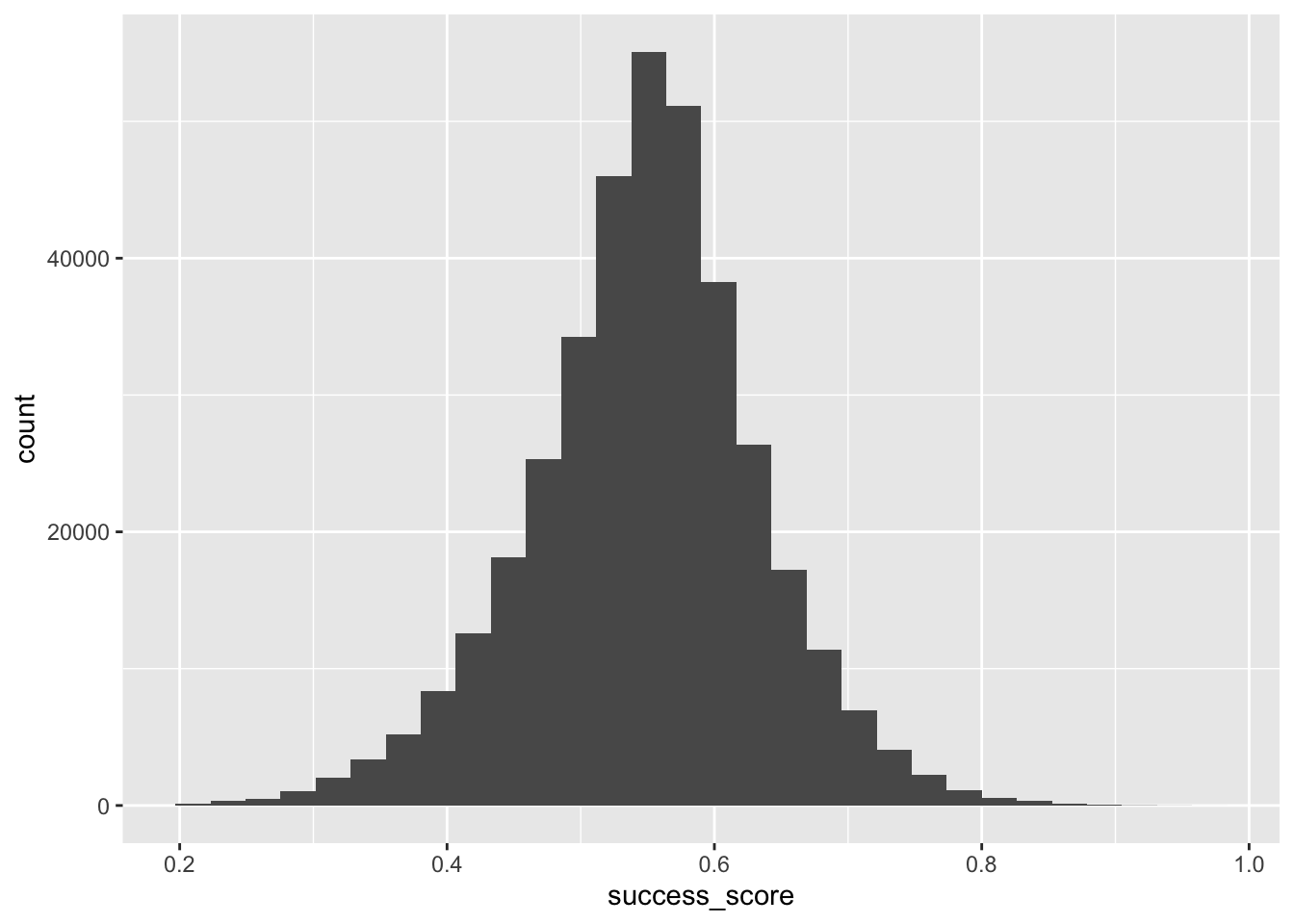

Display Code

summary(TITLE_RATINGS$success_score)

   Min. 1st Qu.  Median    Mean 3rd Qu.    Max. 
 0.2046  0.4987  0.5517  0.5484  0.6000  0.9653

Examining Success by Genre and Decade

In this section, we explore the interplay between film genres and their success across different decades, aiming to uncover trends that can inform a future project. By analyzing the performance of various genres over time, we can identify promising opportunities for an upcoming film.

Display Code

# highest average score
# Biography, Adventure, Animation
TITLE_BASICS |>
  left_join(TITLE_RATINGS, by = "tconst") |>  # Corrected join syntax
  separate_longer_delim(genres, ",") |> 
  group_by(genres) |>  # Group by genres
  summarise(avg_score = mean(success_score, na.rm = TRUE)) |>
  ungroup() |>
  arrange(desc(avg_score)) |>
  head(5)  |>
  gt() |> # create a display table
  tab_header(
    title = "Genres with Top 10 Average Success Scores"
  ) |>
  cols_label( # display column names
    genres = "Genre",
    avg_score = "Average Success Score"
  )

Genres with Top 10 Average Success Scores
Genre	Average Success Score
Biography	0.5739485
Adventure	0.5732288
Animation	0.5721809
Crime	0.5692845
History	0.5671059

The average success scores for the various genres seem fairly close to each other. Instead, we can count the number of success scores greater than the threshold of 0.6 for each genre.

Display Code

# Drama, Comedy, Action
TITLE_BASICS |>
  left_join(TITLE_RATINGS, by = "tconst") |>  # Corrected join syntax
  filter(success_score >= 0.6) |> # greater than threshold
  separate_longer_delim(genres, ",") |> 
  group_by(genres) |>  # Group by genres
  summarise(success_count = n()) |>
  ungroup() |>
  arrange(desc(success_count)) |>
  head(5) |>
  gt() |> # create a display table
  tab_header(
    title = "Genres with Top 10 Average Success Scores"
  ) |>
  cols_label( # display column names
    genres = "Genre",
    success_count = "Number of Success Scores > 0.60"
  )

Genres with Top 10 Average Success Scores
Genre	Number of Success Scores > 0.60
Drama	52577
Comedy	30306
Action	24394
Adventure	19408
Crime	19341

What was the genre with the most “successes” in each decade? What genre consistently has the most “successes”?

Display Code

# Success by genre and decade
success_by_decade <- TITLE_BASICS |>
  left_join(TITLE_RATINGS, by = "tconst") |> 
  filter(success_score >= 0.6) |> 
  mutate(decade = floor(as.integer(startYear) / 10) * 10) |>  # Create a decade column
  separate_longer_delim(genres, ",") |> 
  group_by(decade, genres) |> 
  summarise(success_count = n()) |> 
  ungroup() |>
  arrange(decade, desc(success_count)) 

# Find the genre with the most successes in each decade
top_genre_per_decade <- success_by_decade |>
  group_by(decade) |> 
  slice_max(success_count, n = 1) # select top performing

# Count how many times each genre is the highest in each decade
top_genre_per_decade |>
  group_by(genres) |> 
  summarise(highest_count = n()) |> 
  arrange(desc(highest_count)) |>
  gt() |> # create a display table
  tab_header(
    title = "Number of Times Genres Had the Most Successes of a Decade"
  ) |>
  cols_label( # display column names
    genres = "Genre",
    highest_count = "Frequency"
  )

Number of Times Genres Had the Most Successes of a Decade
Genre	Frequency
Drama	12
Short	3
Comedy	2
Documentary	2
Sport	1

What genre used to reliably produced “successes” and has fallen out of favor?

Display Code

library(ggrepel)
library(ggplot2)

genre_success <- TITLE_BASICS |>
  inner_join(TITLE_RATINGS, by = "tconst") |>
  filter(success_score > 0.6) |>  # Set your success threshold
  filter(!is.na(startYear) & !is.na(success_score)) |>
  separate_longer_delim(genres, ",") |> 
  group_by(genres, startYear) |>
  summarise(success_count = n())

genre_success |>
  ggplot(aes(x = startYear, y = success_count, color = genres)) +
  geom_line(size = 0.5) +       # Use lines to connect points
  geom_point(size = 1) +      # Add points for each data point
  labs(
    title = "Count of Successful Movies by Genre Over Time",
    x = "Year",
    y = "Count of Successful Movies",
    color = "Genre"
  ) +
  theme_minimal() +
  theme(legend.position = "bottom")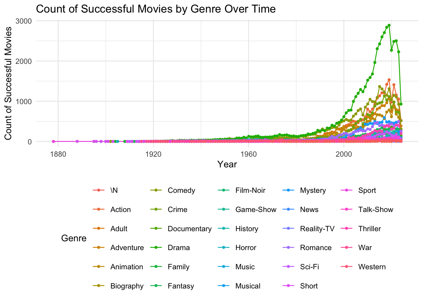

What genre has produced the most “successes” since 2010? It seems that many films just get counted as Dramas with 32923 Dramas.

Display Code

TITLE_BASICS |>
  left_join(TITLE_RATINGS, by = "tconst") |> 
  filter(success_score >= 0.6, startYear >= 2010) |> # filter by 2010
  separate_longer_delim(genres, ",") |> 
  group_by(genres) |> 
  summarise(success_count = n()) |> 
  ungroup() |>
  arrange(desc(success_count)) |>
  head(5) |>
  gt() |> # create a display table
  tab_header(
    title = "Success Count by Genre"
  ) |>
  cols_label( # display column names
    genres = "Genre",
    success_count = "Success Count"
  )

Success Count by Genre
Genre	Success Count
Drama	32923
Comedy	16142
Action	15961
Crime	12626
Adventure	11665

Display Code

recent_top_genres <- TITLE_BASICS |>
  left_join(TITLE_RATINGS, by = "tconst") |> 
  filter(success_score >= 0.6, startYear >= 2010) |> 
  separate_longer_delim(genres, ",") |> 
  group_by(genres) |> 
  summarise(success_count = n()) |> 
  ungroup() |>
  arrange(desc(success_count)) |>
  head(5)

recent_top_genres |>
  ggplot(aes(x = genres, y = success_count, fill = genres)) +
  geom_bar(stat="identity") +
  labs(
    title = "Count of Successful Movies by Genre Over Time",
    x = "Genre",
    y = "Count of Successful Movies",
    color = "Genre"
  ) +
  theme_minimal() +
  theme(legend.position = "bottom")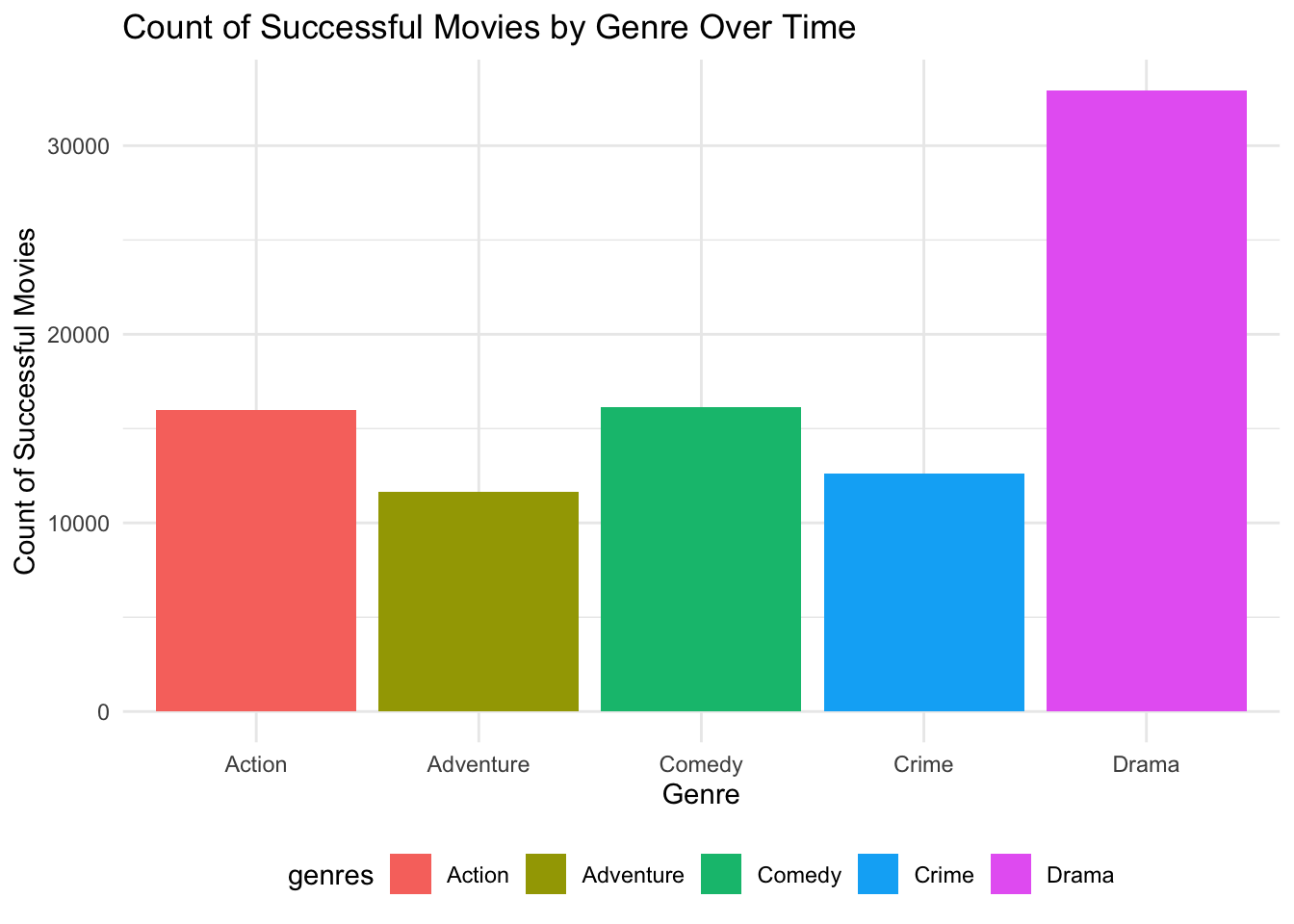

Within the Drama genre, what were the most successful movies? It turns out the top movies we saw before all fall within the Drama genre as well.

Display Code

TITLE_RATINGS |> 
  arrange(desc(success_score)) |>  
  left_join(TITLE_BASICS, join_by("tconst" )) |> 
  filter(titleType == 'movie') |> 
  separate_longer_delim(genres, ",") |> 
  filter(genres == "Drama") |>
  select(primaryTitle, success_score, averageRating, numVotes) |>
  head(10) |>
  gt() |> # create a display table
  tab_header(
    title = "Most Successful Drama Movies"
  ) |>
  cols_label( # display column names
    primaryTitle = "Title",
    success_score = "Success Score",
    averageRating = "Average Rating",
    numVotes = "Number of Votes"
  )

Most Successful Drama Movies
Title	Success Score	Average Rating	Number of Votes
The Shawshank Redemption	0.9648769	9.3	2942823
The Dark Knight	0.9495972	9.0	2922922
The Godfather	0.9477853	9.2	2051186
The Lord of the Rings: The Return of the King	0.9371353	9.0	2013824
Pulp Fiction	0.9359758	8.9	2260017
Fight Club	0.9326142	8.8	2374722
The Lord of the Rings: The Fellowship of the Ring	0.9326021	8.9	2043202
Forrest Gump	0.9315685	8.8	2301630
Schindler's List	0.9267397	9.0	1475891
The Godfather Part II	0.9246497	9.0	1386499

What about the second most successful genre, Comedy?

Display Code

TITLE_RATINGS |> 
  arrange(desc(success_score)) |>  
  left_join(TITLE_BASICS, join_by("tconst" )) |> 
  filter(titleType == 'movie') |> 
  separate_longer_delim(genres, ",") |> 
  filter(genres == "Comedy") |>
  select(primaryTitle, success_score, averageRating, numVotes) |>
  head(5) |>
  gt() |> # create a display table
  tab_header(
    title = "Most Successful Comedy Movies"
  ) |>
  cols_label( # display column names
    primaryTitle = "Title",
    success_score = "Success Score",
    averageRating = "Average Rating",
    numVotes = "Number of Votes"
  )

Most Successful Comedy Movies
Title	Success Score	Average Rating	Number of Votes
Django Unchained	0.9069468	8.5	1729019
Back to the Future	0.8982525	8.5	1333279
The Wolf of Wall Street	0.8897217	8.2	1620302
The Intouchables	0.8867587	8.5	945572
Life Is Beautiful	0.8842202	8.6	754383

Successful Personnel in the Genre

As I develop my team, I want to consider the benefits of pairing an older, established actor—someone with over 20 successful titles—to lend credibility and experience, alongside an up-and-coming actor who can bring fresh energy and appeal to a younger audience. This combination can create a dynamic synergy that enhances the project’s overall impact.

When working with NAME_BASICS, I can only have alive personnel on my team. Here, I am creating a new data frame called ALIVE_NAME_BASICS.

Display Code

ALIVE_NAME_BASICS <- NAME_BASICS |>
  filter(birthYear >= 1916, is.na(deathYear)) # Can only have alive personnel on my team
sample_n(ALIVE_NAME_BASICS, 1000) |>
  DT::datatable()

I will aso identify titles with a success score greater than 0.6 in SUCCESSFUL_TITLES.

Display Code

#Successful Movies Dataset
SUCCESSFUL_TITLES <- TITLE_BASICS |>
  left_join(TITLE_RATINGS, by = "tconst") |>
  filter(success_score >= 0.6)
sample_n(SUCCESSFUL_TITLES, 1000) |>
  DT::datatable()

Established Drama Actors & Actresses

Display Code

# actor
TITLE_PRINCIPALS |>
  filter(category == "actor") |>
  filter(tconst %in% SUCCESSFUL_TITLES$tconst) |>
  select(tconst, nconst) |>
  inner_join(ALIVE_NAME_BASICS, by = "nconst") |>
  inner_join(SUCCESSFUL_TITLES, by = "tconst") |>
  filter(titleType == "movie") |>
  separate_longer_delim(genres, ",") |> 
  filter(genres == "Drama") |>
  group_by(primaryName) |>
  summarise(
    success_count = n(),
    mean_success_score = mean(success_score, na.rm = TRUE)  # Ensure NA values are ignored
  ) |>
  filter(success_count >= 20) |>
  arrange(desc(mean_success_score), desc(success_count)) |>
  head(5)|>
  gt() |> # create a display table
  tab_header(
    title = "Top 5 Drama Actors"
  ) |>
  cols_label( # display column names
    primaryName = "Actor Name",
    success_count = "Success Count",
    mean_success_score = "Mean Success Score"
  )

Top 5 Drama Actors
Actor Name	Success Count	Mean Success Score
Brad Pitt	31	0.7833171
Leonardo DiCaprio	28	0.7801242
Christian Bale	38	0.7641907
Ryan Gosling	21	0.7620046
Tom Hanks	38	0.7595574

Display Code

# actor
TITLE_PRINCIPALS |>
  filter(category == "actress") |>
  filter(tconst %in% SUCCESSFUL_TITLES$tconst) |>
  select(tconst, nconst) |>
  inner_join(ALIVE_NAME_BASICS, by = "nconst") |>
  inner_join(SUCCESSFUL_TITLES, by = "tconst") |>
  filter(titleType == "movie") |>
  separate_longer_delim(genres, ",") |> 
  filter(genres == "Drama") |>
  group_by(primaryName) |>
  summarise(
    success_count = n(),
    mean_success_score = mean(success_score, na.rm = TRUE)  # Ensure NA values are ignored
  ) |>
  filter(success_count >= 20) |>
  arrange(desc(mean_success_score), desc(success_count)) |>
  head(5)|>
  gt() |> # create a display table
  tab_header(
    title = "Top 5 Drama Actresses"
  ) |>
  cols_label( # display column names
    primaryName = "Actor Name",
    success_count = "Success Count",
    mean_success_score = "Mean Success Score"
  )

Top 5 Drama Actresses
Actor Name	Success Count	Mean Success Score
Scarlett Johansson	30	0.7471914
Frances McDormand	24	0.7253185
Emily Blunt	23	0.7252131
Jessica Chastain	24	0.7219137
Natalie Portman	26	0.7205248

Up and Coming Actors & Actresses

To find up and coming actors, I tried a couple of ways to define the criteria for “up and coming”. What if we consider mean success score? We could find top scoring actors but with low success counts.

Display Code

# actor
TITLE_PRINCIPALS |>
  filter(category == "actor") |>
  filter(tconst %in% SUCCESSFUL_TITLES$tconst) |>
  select(tconst, nconst) |>
  inner_join(ALIVE_NAME_BASICS, by = "nconst") |>
  inner_join(SUCCESSFUL_TITLES, by = "tconst") |>
  filter(titleType == "movie") |>
  separate_longer_delim(genres, ",") |> 
  filter(genres == "Drama") |>
  group_by(primaryName) |>
  summarise(
    success_count = n(),
    mean_success_score = mean(success_score, na.rm = TRUE)  # Ensure NA values are ignored
  ) |>
  arrange(desc(mean_success_score), desc(success_count)) |>
  head(5) |>
  gt() |>
  tab_header(
    title = "Top Scoring Actors with Low Success Counts"
  ) |>
  cols_label( # display column names
    primaryName = "Actor Name",
    success_count = "Success Count",
    mean_success_score = "Mean Success Score"
  )

Top Scoring Actors with Low Success Counts
Actor Name	Success Count	Mean Success Score
Michael Conner Humphreys	1	0.9315685
John Bach	2	0.9303864
Sala Baker	4	0.9303610
Jonathan Sagall	1	0.9267397
Shmuel Levy	1	0.9267397

Michael Conner Humphreys has only been in 1 film where he played young Forrest Gump. This does not seem like the best way to define up and coming. I do want someone with a higher success count. What if I limit it to between 5 and 10 successful titles.

Display Code

TITLE_PRINCIPALS |>
  filter(category == "actor") |>
  filter(tconst %in% SUCCESSFUL_TITLES$tconst) |>
  select(tconst, nconst) |>
  inner_join(ALIVE_NAME_BASICS, by = "nconst") |>
  inner_join(SUCCESSFUL_TITLES, by = "tconst") |>
  separate_longer_delim(genres, ",") |> 
  filter(genres == "Drama") |>
  filter(titleType == "movie", startYear >=2020) |>
  group_by(primaryName) |>
  summarise(
    success_count = n(),
    mean_success_score = mean(success_score, na.rm = TRUE)  # Ensure NA values are ignored
  ) |>
  filter(success_count >=5 & success_count <=10) |> # 5 to 10 successful titles
  arrange(desc(mean_success_score), desc(success_count)) |>
  head(10) |>
  gt() |>
  tab_header(
    title = "Actors with High Success Scores and Between 5-10 Successful Titles Since 2020"
  ) |>
  cols_label( # display column names
    primaryName = "Actress Name",
    success_count = "Success Count",
    mean_success_score = "Mean Success Score"
  )

Actors with High Success Scores and Between 5-10 Successful Titles Since 2020
Actress Name	Success Count	Mean Success Score
Timothée Chalamet	5	0.8000488
Colin Farrell	6	0.7626842
Sahil Vaid	5	0.7508455
Jeffrey Wright	5	0.7449358
Mark Rylance	5	0.7401355
Achyuth Kumar	7	0.7290892
Tom Hanks	7	0.7270197
Ajay Devgn	9	0.7232701
Rao Ramesh	6	0.7230589
Johnny Flynn	5	0.7157819

Tom Hanks… I don’t think I could consider him an up and coming actor. Let us adjust again. It seems like the startYear lowers the success count. It only counts for recent movies and so established actors show up too because their earlier successes are not counted. Does up and coming mean young or just that their first movie was recent? I think older personell can be up and coming if they are just coming into the scene. Let’s try looking at the minimum start year of their first titles and actors with a number of successes.

Display Code

TITLE_PRINCIPALS |>
  filter(category == "actor") |>
  select(tconst, nconst) |>
  right_join(ALIVE_NAME_BASICS, by = "nconst") |>
  left_join(TITLE_BASICS, by = "tconst") |>
  left_join(TITLE_RATINGS, by = "tconst") |>
  separate_longer_delim(genres, ",") |> 
  filter(genres == "Drama", titleType == "movie") |>
  select(primaryName, primaryTitle, startYear, genres, success_score) |>
  filter(success_score >= 0.6) |>  # Filter by success score
  group_by(primaryName) |>  # group by actor
  summarise(
    debut_year = min(startYear, na.rm = TRUE),  # Compute first movie they did here
    success_count = n(), # count succeses 
    mean_success_score = mean(success_score, na.rm = TRUE), # find mean success score
    .groups = 'drop'
  ) |>
  filter(debut_year >= 2015, success_count >= 5 & success_count <= 10) |>
  arrange(desc(mean_success_score), desc(success_count)) |>
  head(5) |>
  gt() |>
  tab_header(
    title = "Up and Coming Actors"
  ) |>
  cols_label( # display column names
    primaryName = "Name",
    debut_year = "Year of First Movie",
    success_count = "Success Count",
    mean_success_score = "Mean Success Score"
  )

Up and Coming Actors
Name	Year of First Movie	Success Count	Mean Success Score
Anthony Ramos	2018	5	0.7734428
Noah Jupe	2017	7	0.7565397
Barry Keoghan	2017	8	0.7535545
Dave Bautista	2015	7	0.7352465
Leslie Odom Jr.	2019	5	0.7348193

Selecting Anthony Ramos, Noah Jupe, and Barry Keoghan from this list, I would consider them lesser known actors who were a part of successful films.

Combinations of Personnel

Actor/director pairs who have been successful together

Display Code

# Filter actors and directors first
actors_df <- TITLE_PRINCIPALS |>
  filter(category %in% c("actor", "actress")) |>
  select(tconst, nconst)

directors_df <- TITLE_PRINCIPALS |>
  filter(category == "director") |>
  select(tconst, nconst)

# Join actors and directors to create combinations
actor_director_pairs <- actors_df |>
  inner_join(directors_df, by = "tconst", suffix = c("_actor", "_director"), relationship = "many-to-many")

actor_director_names <- actor_director_pairs |>
  inner_join(ALIVE_NAME_BASICS, by = c("nconst_actor" = "nconst"), relationship = "many-to-many") |> # join to names
  rename(actor_name = primaryName) |>
  inner_join(ALIVE_NAME_BASICS, by = c("nconst_director" = "nconst"), relationship = "many-to-many") |> # join to names
  rename(director_name = primaryName) |>
  inner_join(TITLE_BASICS, by = "tconst") |> # join with titles
  inner_join(TITLE_RATINGS, by = "tconst") # join with ratings

actor_director_names |> 
  group_by(actor_name, director_name) |> # group by actor_name and director_name combinations
  summarise(
    success_count = n(), # count the number of times they've worked together
    mean_success_score = mean(success_score, na.rm = TRUE)) |> # find the mean success score
  filter(mean_success_score > 0.60) |>
  select(actor_name, director_name, success_count, mean_success_score) |>
  arrange(desc(success_count), desc(mean_success_score)) |>
  head(10)

# A tibble: 10 × 4
# Groups:   actor_name [10]
   actor_name       director_name        success_count mean_success_score
   <chr>            <chr>                        <int>              <dbl>
 1 Trey Parker      Trey Parker                    888              0.669
 2 Matt Stone       Trey Parker                    866              0.670
 3 Masako Nozawa    Daisuke Nishio                 466              0.612
 4 Hank Azaria      Mark Kirkland                  350              0.615
 5 Dan Castellaneta Mark Kirkland                  346              0.614
 6 Mona Marshall    Trey Parker                    338              0.674
 7 Harry Shearer    Mark Kirkland                  336              0.615
 8 Sam Marin        John Davis Infantino           301              0.685
 9 Nancy Cartwright Mark Kirkland                  281              0.614
10 William Salyers  John Davis Infantino           274              0.688

I am getting mostly voice actors in the result above. My guess is this is due to episodes and tv series having a higher count. It may help to filter out the TV episodes. We can see how directors of TV series that work with the same actors multiple times may skew the success count.

Display Code

TITLE_BASICS |>
  group_by(titleType) |>
  summarize(count = n())

# A tibble: 10 × 2
   titleType     count
   <chr>         <int>
 1 movie        131662
 2 short         16656
 3 tvEpisode    155722
 4 tvMiniSeries   5907
 5 tvMovie       15007
 6 tvSeries      29789
 7 tvShort         410
 8 tvSpecial      3045
 9 video          9332
10 videoGame      4668

Top 10 Actor/Actress and Director Pairs in Drama Genre

Display Code

actor_director_names |> 
  filter(titleType == "movie") |> # filter for movies so results are not skewed by number of episodes
  separate_longer_delim(genres, ",") |>
  filter(genres == "Drama") |> # filter by Drama
  group_by(actor_name, director_name) |> # group by actor_name and director_name combinations
  summarise(
    success_count = n(), # count the number of times they've worked together
    mean_success_score = mean(success_score, na.rm = TRUE)) |> # find the mean success score
  filter(mean_success_score > 0.60, success_count > 5) |>
  arrange(desc(mean_success_score), desc(success_count)) |>
  head(10)

# A tibble: 10 × 4
# Groups:   actor_name [10]
   actor_name          director_name     success_count mean_success_score
   <chr>               <chr>                     <int>              <dbl>
 1 Christian Bale      Christopher Nolan             7              0.913
 2 Robert De Niro      Martin Scorsese               8              0.809
 3 Ethan Hawke         Richard Linklater             7              0.766
 4 Prabhas             S.S. Rajamouli                6              0.757
 5 Frank Welker        Don Bluth                     6              0.757
 6 Penélope Cruz       Pedro Almodóvar               6              0.739
 7 Tony Leung Chiu-wai Kar-Wai Wong                  7              0.735
 8 Woody Allen         Woody Allen                   7              0.729
 9 Clint Eastwood      Clint Eastwood               18              0.728
10 Megumi Hayashibara  Kazuya Tsurumaki             14              0.723

What if we look at a specific director to see what actors and actresses they work well with. For example, if I wanted Steven Spielberg. Who has he worked well with in the past?

Display Code

actor_director_names |> 
  filter(titleType == "movie") |> # filter for movies so results are not skewed by number of episodes
  filter(director_name == "Steven Spielberg") |>
  group_by(actor_name, director_name) |> # group by actor_name and director_name combinations
  summarise(
    success_count = n(), # count the number of times they've worked together
    mean_success_score = mean(success_score, na.rm = TRUE)) |> # find the mean success score
  select(actor_name, success_count, mean_success_score) |>
  arrange(desc(success_count), desc(mean_success_score)) |>
  head(5)

# A tibble: 5 × 3
# Groups:   actor_name [5]
  actor_name    success_count mean_success_score
  <chr>                 <int>              <dbl>
1 Tom Hanks                 5              0.832
2 Harrison Ford             4              0.830
3 Mark Rylance              4              0.781
4 Dan Aykroyd               4              0.669
5 Simon Pegg                3              0.801

Now let’s look at people the director has worked with at least twice.

Display Code

actor_director_names |> 
  filter(titleType == "movie") |> # filter for movies so results are not skewed by number of episodes
  filter(director_name == "Steven Spielberg") |>
  group_by(actor_name, director_name) |> # group by actor_name and director_name combinations
  summarise(
    success_count = n(), # count the number of times they've worked together
    mean_success_score = mean(success_score, na.rm = TRUE)) |> # find the mean success score
  filter(success_count >= 2) |> # worked with multiple times (at least twice)
  select(actor_name, success_count, mean_success_score) |>
  arrange(desc(mean_success_score), desc(success_count)) |>
  head(5) |>
  gt() |>
  tab_header(
    title = "Actors & Actresses Steven Spielberg Worked With"
  ) |>
  cols_label( # display column names
    actor_name = "Actor/Actress",
    success_count = "Success Count",
    mean_success_score = "Mean Success Score"
  )

Actors & Actresses Steven Spielberg Worked With
Success Count	Mean Success Score
Giovanni Ribisi
2	0.9076895
Vic Tablian
2	0.8852299
John Rhys-Davies
2	0.8761031
Caroline Goodall
2	0.8435231
Tom Hanks
5	0.8319899

Nostalgia and Remakes

The classic movie I propose to remake is The Princess Bride. Remaking The Princess Bride, a classic with an 8 IMDb rating, taps into a well-loved story while allowing us to introduce fresh talent, including original cast cameos, to engage both longtime fans and new audiences. The original has a large number of IMDb ratings, a high average rating, and has not been remade in the past 25 years. A Princess Bride Home Movie was created during COVID, a miniseries shot on phones from home, but a full film remake would be very successful.

Display Code

TITLE_BASICS |>
  filter(primaryTitle == "The Princess Bride")|>
  inner_join(TITLE_RATINGS, by = "tconst") |>
  select(primaryTitle, averageRating, numVotes, success_score) |>
  gt() |>
  tab_header(
    title = "The Princess Bride"
  ) |>
  cols_label( # display column names
    primaryTitle = "Title",
    averageRating = "Average Rating",
    numVotes = "Number of Votes",
    success_score = "Success Score"
  )

The Princess Bride
Title	Average Rating	Number of Votes	Success Score
The Princess Bride	8	456797	0.8373338

Successful Genres The Princess Bride is a film filled with Drama, Action, and Comedy, three of the top performing genres.

Display Code

recent_top_genres <- TITLE_BASICS |>
  left_join(TITLE_RATINGS, by = "tconst") |> 
  filter(success_score >= 0.6) |> 
  separate_longer_delim(genres, ",") |> 
  filter(genres %in% c("Drama", "Comedy", "Action")) |>
  group_by(genres, startYear) |>  # Group by genres and startYear
  summarise(success_count = n(), .groups = 'drop') |> 
  ungroup() |>
  arrange(startYear, desc(success_count))

Display Code

ggplot(recent_top_genres, aes(x = startYear, y = success_count, fill = genres)) +
  geom_bar(stat = "identity") +
  labs(
    title = "Growth of Successful Movies by Genre Over Time",
    x = "Year",
    y = "Count of Successful Movies",
    fill = "Genre"
  ) +
  theme_minimal() +
  theme(legend.position = "bottom") +
  facet_wrap(~ genres, scales = "free_y")  # Create separate plots for each genre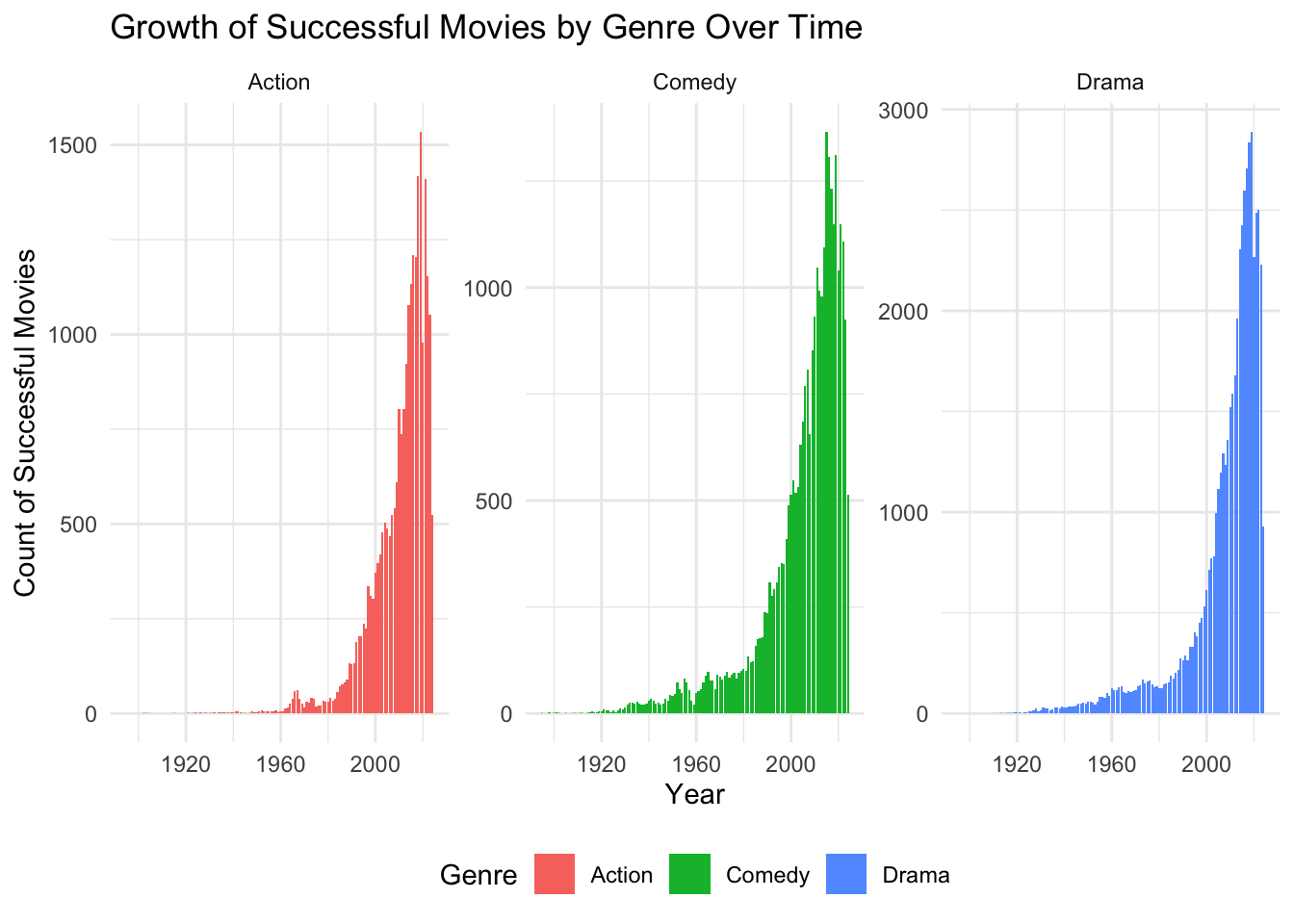

Key Personnel Let’s confirm whether key actors, directors, or writers from the original are still alive.

Display Code

TITLE_PRINCIPALS |>
  filter(tconst == "tt0093779") |>
  inner_join(NAME_BASICS, by = "nconst") |>
  filter(category %in% c("actor", "actress", "director", "writer")) |>
  select(primaryName, category, characters, deathYear) |>
  gt() |> # create a display table
  tab_header(
    title = "Key Personnel"
  ) |>
  cols_label( # display column names
    primaryName = "Name",
    category = "Role",
    characters = "Characters",
    deathYear = "Death Year"
  )

Key Personnel
Name	Role	Characters	Death Year
Cary Elwes	actor	["Westley"]	NA
Mandy Patinkin	actor	["Inigo Montoya"]	NA
Robin Wright	actress	["The Princess Bride"]	NA
Christopher Guest	actor	["Count Rugen"]	NA
Wallace Shawn	actor	["Vizzini"]	NA
André René Roussimoff	actor	["Fezzik"]	1993
Fred Savage	actor	["The Grandson"]	NA
Peter Falk	actor	["The Grandfather"]	2011
Peter Cook	actor	["The Impressive Clergyman"]	1995
Rob Reiner	director	\N	NA
William Goldman	writer	\N	2018

Proven Director <a

Renowned for his ability to capture magic in storytelling, Steven Spielberg is ideal for reimagining this beloved classic. With Steven Spielberg, we can get a balance of heartfelt storytelling and commercial success, making this project a compelling remake. His success in genres such as Drama and Action fit well with The Princess Bride.

Display Code

NAME_BASICS |>
  filter(primaryName == 'Steven Spielberg') |>
  separate_longer_delim(knownForTitles, ",") |> 
  left_join(TITLE_BASICS, by = c("knownForTitles" = "tconst")) |> 
  left_join(TITLE_RATINGS, by = c("knownForTitles" = "tconst")) |>
  select(primaryName, primaryTitle, success_score, averageRating, numVotes) |>
  arrange(desc(success_score)) |>
  gt() |> # create a display table
  tab_header(
    title = "Steven Spielberg    Project Scores"
  ) |>
  cols_label( # display column names
    primaryName = "Name",
    primaryTitle = "Title",
    success_score = "Success Score",
    averageRating = "Average Rating",
    numVotes = "Number of Votes"
  )

Steven Spielberg Project Scores
Name	Title	Success Score	Average Rating	Number of Votes
Steven Spielberg	Schindler's List	0.9267397	9.0	1475891
Steven Spielberg	Saving Private Ryan	0.9076895	8.6	1521594
Steven Spielberg	Raiders of the Lost Ark	0.8852299	8.4	1049518
Steven Spielberg	E.T. the Extra-Terrestrial	0.8313398	7.9	443655

Steven Spielberg has consistently directed successful movies for over 5 decades.

Display Code

spielberg_success <- TITLE_PRINCIPALS |>
filter(nconst %in% NAME_BASICS$nconst[NAME_BASICS$primaryName == "Steven Spielberg"]) |>
  inner_join(TITLE_BASICS, by = "tconst") |>
  inner_join(TITLE_RATINGS, by = "tconst") |>
  select(primaryTitle, startYear, success_score) |>
  distinct() |>  # Remove duplicates
  mutate(successful = ifelse(success_score >= 0.6, 1, 0)) |>
  group_by(startYear) |>
  summarise(success_count = sum(successful), .groups = 'drop') |>
  filter(success_count > 0) |>  # Only keep years with successful films
  arrange(startYear)

Display Code

# Plotting
ggplot(spielberg_success, aes(x = startYear, y = success_count)) +
  geom_line(color = "blue", size = .5) +
  geom_point(color = "blue", size = 1) +
  labs(title = "Number of Successful Films Directed by Steven Spielberg Over Time",
       x = "Year",
       y = "Number of Successful Films") +
  scale_y_continuous(limits = c(0, NA)) +  # Set y-axis to start at 0
  theme_minimal()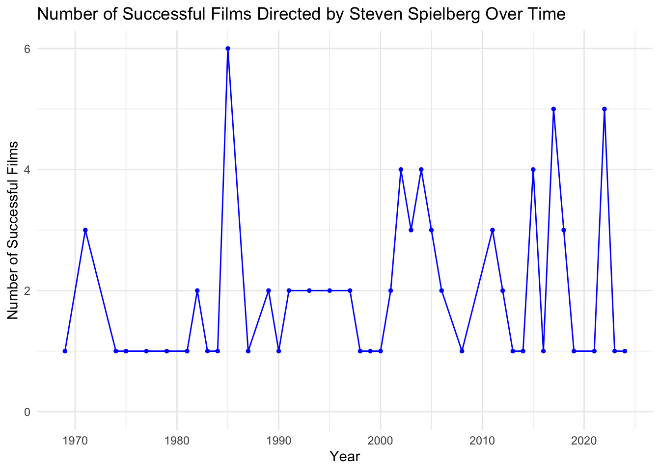

Casting The original actress, Robin Wright, who played The Princess Bride has previously worked with Tom Hanks in the successful film Forrest Gump. However, it might be a good idea to cast some up and coming actors and actresses as leads to attract newer audience. We can keep Wallace Shawn as Vizzini for fans and a nod towards the original classic. By casting Mille Bobby Brown as The Princess Bride and Noah Jupe as Westley. Noah is known for his performances in A Quiet Place and Honey Boy, Jupe brings a fresh energy and charm suitable for the role of Westley. Timothée Chalamet could be cast as Inigo Montoya. His performances in Dune: Part Two and Part One make him an excellent choice for the iconic role of Inigo, seeking vengeance for his father.

Elevator Pitch

From the visionary mind of Steven Spielberg comes a timeless tale of adventure and romance, The Princess Bride. Featuring the talented Noah Jupe as Westley and the dynamic Millie Bobby Brown as Buttercup, this re-imagining will delight both old fans and new. With Timothée Chalamet as the iconic Inigo Montoya and Wallace Shawn reprising his role as Vizzini, alongside the incredible Julianne Moore, this film is a story of love, bravery, and the magic of storytelling—coming soon to theaters near you!

This remake promises to capture the heart of the original while inviting audiences into a fresh, enchanting cinematic experience.